Blog: Causal inference using graphs
DAG intro Heading link
Some of the most critical research questions involve estimating causal effects, not simply correlations or associations. It is not uncommon to see an everything-but-the-kitchen-sink approach, where every available covariate is included in the model. Intuitively, it would seem that these adjustments control for confounds, and thus improve our estimates. However, as we saw in our previous post about Simpson’s paradox, sometimes conditioning on a variable actually destroys our causal estimates. In that post, we saw an example where including blood pressure in the model would cause us to think that a harmful medicine was actually helpful, a very dangerous conclusion!
Deciding which variables to include requires us to think about cause and effect. In this blog post, we explain how to represent causal relationships between variables using a directed acyclic graph (DAG), and how to use this type of DAG to determine which variables to include in a model when estimating causal effects. A graph, specifically in the sense of graph theory, is a set of nodes and a set of edges (connections between the nodes). Directed means that there is an order to the edges, that is a connection might go from node X to node Y but not from node Y to node X. Finally, acyclic means that there is no way to follow a path from one node back to the same node.
In our DAGs, we will use nodes to represent variables (observed or unobserved), and edges to represent causal relationships between the variables. For example, if a medicine causes high blood pressure, then there will be an edge going from medicine to blood pressure. Note that the edge doesn’t specify anything about the association beyond a causal effect. There could be a simple linear relationship or a complex non-linear relationship. It will be up to you to model the relationship; the DAG will simply let you know which variables to include or exclude when estimating causal effects.
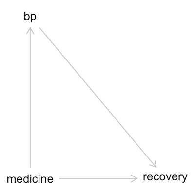
Let’s start by considering the example from the previous blog post about blood pressure, medicine, and recovery. In our first scenario, the medicine causes high blood pressure, people with high blood pressure are less likely to recover, and people who receive the medicine are more likely to recover. This results in the DAG shown below:
DAG 2 Heading link
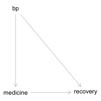
In our second scenario, the causal relationship between blood pressure and medicine is flipped: people with high blood pressure are more likely to receive medicine, people with high blood pressure are less likely to recover, and people who receive medicine are more likely to recover. This results in the DAG shown below:
DAG 2 Heading link
Keep in mind that both of these DAGs can be compatible with the same data (for example, see the table below). You may need to use additional data or domain knowledge to determine which model is more realistic.
title Heading link
| low bp control | low bp treated | high bp control | high bp treated | |
|---|---|---|---|---|
| recovered | 80 | 10 | 40 | 50 |
| sick | 20 | 0 | 60 | 50 |
Encoding DAGs in Daggity Heading link
Once you have a DAG, you can determine which variables to include in your model to ensure proper estimation of causal effects. There is a complicated set of rules you can follow to compute this by hand, but it is easier and less error-prone to use software like DAGitty to automate the calculation. DAGitty exists as a web app as well as an R package. Here we show a brief example using the R package to determine which variables to include in the model and which to exclude.
Let’s start with the first DAG. We store the DAG in a variable g1, writing each edge as cause → effect:
g1 = dagitty("dag{
  bp -> recovery
  medicine -> bp
  medicine -> recovery
}")
Next, we use the adjustmentSets function to determine what to adjust for when estimating the causal effect that the medicine has on recovery. In the function, we set exposure to “medicine”, since that is the exposure whose causal effect we want to estimate, and we set outcome to “recovery” since we want to know the causal effect of “medicine” on “recovery”.
adjustmentSets(g1, exposure="medicine", outcome="recovery")

output: {}
Upon running the function, DAGitty returns an empty set of braces, telling us not to control for anything, as we saw in the previous blog post. Now let’s consider the second DAG:
g2 = dagitty("dag{
  bp -> medicine
  bp -> recovery
  medicine -> recovery
}")

adjustmentSets(g2, exposure="medicine", outcome="recovery")

output: { bp }
In this case we see that DAGitty tells us to control for blood pressure, much like we controlled for age in the previous post.
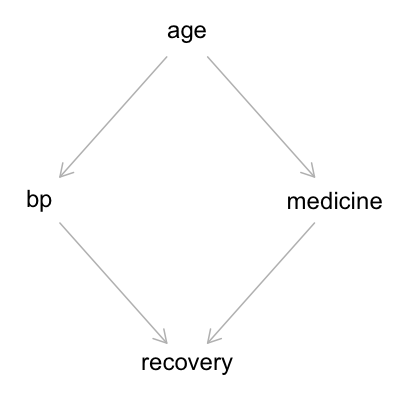
Now let’s consider two more complex causal relationships. In our third scenario, we consider the following: older people have higher blood pressure and are more likely to receive treatment, people with higher blood pressure are less likely to recover, and people who receive treatment are more likely to recover. The DAG below shows this set of causal relationships:
DAG 3 and 4 Heading link
g3 = dagitty("dag{
  age -> bp
  age -> medicine
  bp -> recovery
  medicine -> recovery
}")

adjustmentSets(g3, exposure="medicine", outcome="recovery")

output:
 { bp }
 { age }
DAGitty gives us two adjustment sets in this case: we can either adjust for age, or adjust for blood pressure. This flexibility can be useful in cases where some of our variables are unobserved.
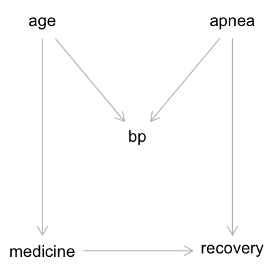
Now our final scenario. As people get older, their blood pressure increases. Sleep apnea also causes high blood pressure. Older people are more likely to receive medicine. People with sleep apnea are less likely to recover, and people who receive medicine are more likely to recover. The DAG below shows this set of causal relationships:
Conclusion Heading link
g4 = dagitty("dag{
  age -> medicine
  age -> bp
  apnea -> bp
  apnea -> recovery
  medicine -> recovery
}")

adjustmentSets(g4, exposure="medicine", outcome="recovery")

output: {}
Here DAGitty tells us that we do not want to include any of these variables in our model. Note that we cannot simply use temporal ordering as a heuristic for determining causal relationships. In our final scenario, elevated blood pressure precedes treatment, but should not be included in the model. We must explicitly model the causal structure.
If you are interested in using causal DAGs in your own research, you can find more resources for learning about DAGs and DAGitty here, or reach out to ACER for our data science consulting services.